Mirta Ciocca1 ID·
Ricardo Mastai1 ID·
Arturo Cagide2 ID
1 German Hospital of Buenos Aires.
2 Italian Hospital of Buenos
Aires.
City of Buenos Aires, Argentina.
Acta Gastroenterol Latinoam 2025;55(2):79-87
Received: 05/04/2025 /
Accepted: 06/02/2025 / Published online: 30/06/2025
/
https://doi.org/10.52787/agl.v55i2.489
At a center specializing in liver diseases, a new drug ("Tx. X") has been used to treat portal hypertension. The professionals are convinced that the drug reduces gastrointestinal bleeding associated with this syndrome.
A statistical analysis shows that with Tx. X, there was a significant decrease in that complication, with p < 0.05.
But a question arises: Did only patients with better clinical conditions and
favorable prognosis, such as younger age, lower degree of portal hypertension, or an absence of
thrombocytopenia, receive the treatment?.
If so, is the p < 0.05 due to the treatment or because the
intervention acted as a "selector" of a lower-risk population?
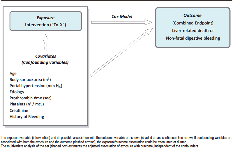
Figure 1 illustrates a fictional observational study, in which the exposure variable (the research objective) could be associated with the evolution variable (the end point or “outcome”) or with a certain number of confounders (or covariates) that can affect that association.
For instance, as previously mentioned, if an intervention that can favorably modify the outcome –in this case, liver-related mortality or non-fatal gastrointestinal bleeding- is preferentially indicated for patients with a higher platelet counts or less severe disease, the benefit could be due to the treatment or the fact that the procedure "selected" individuals with a lower bleeding risk. Note that this detailed condition requires the association of confounders with the intervention.
In other words, any imbalance in the prevalence of confounders between comparison groups can distort the target association. Thus, when only the relationship between the intervention and the outcome is considered using univariate or unadjusted analysis, the resulting p value may have no clinical significance with regard to the treatment effect.
This situation does not affect randomized (experimental) trials because the decision to intervene is based on chance rather than medical necessity, ensuring balanced distribution of confounders in both intervention and control groups. However, randomization can occasionally fail, especially in small samples.
The usual procedure to address this issue in a follow-up trial is the multivariate method of logistic regression or Cox proportional hazards model (hereafter, “Cox model”).
With this methodology, the exposure variable and the confounders (selected for their isolated statistical association or the bibliographic contribution -independent variables-) are analyzed together (Figure 1). This procedure is usually referred to as adjustment. In multivariate analysis, if the exposure variable is statistically significant in relation to the outcome variable (dependent variable), it is concluded that this association is not conditional on confounders.
However, multivariate analysis requires a specific ratio of independent variables to outcome variable prevalence/incidence, which limits the applicability of this methodology under certain conditions.
Figure 1. Multivariate Study
Propensity Score (PS)
A second statistical methodology is balancing the confounders so that they are equal between the intervention and control groups.
Figure 2 illustrates the procedure. First, the association between confounders (now independent variables) and the exposure (now dependent variable) is estimated statistically using multivariate analysis (logistic regression in this case).
The Propensity Score (PS) which is the probability of being exposed to the intervention independently of the confounders, is derived from this analysis. Individuals with similar PS should have an equal probability of receiving the treatment under investigation, whether or not they actually received it.
An advantage of PS over multivariate analysis is that the number of independent variables is not limited by the prevalence of the outcome, since the intervention group, will always have a sufficient number of observations.
Figure 2. Propensity Score and Derived Analyses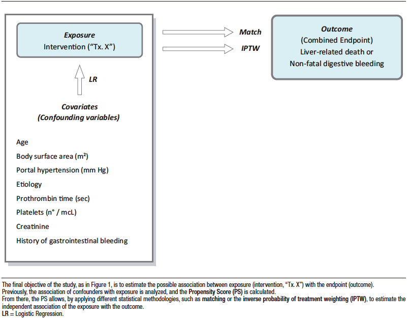
Exposure and Outcome Variables
There is some debate about which variables should be included in the PS calculation. In general, they should include all those that the investigator considers to condition a given treatment or intervention. In principle, outcome variables should also be included.
However, as in any multivariate analysis, only known and available independent variables are considered, which can result in flawed PS prediction of exposure to the treatment or intervention.
The ROC curve can be applied to calculate the accuracy of the model in the calculation of PS. Although there are discrepancies in the value considered adequate, most authors consider 0.80 acceptable.
PS, Covariate Adjustment, and Outcome Estimation
Matching
Following the above methodology, each individual will be characterized by a certain PS according to his or her baseline characteristics or confounders. Some individuals in the intervention group will have a similar PS to those in the control group, so that it is possible to match patients in both groups according to their PS (Figure 3).
Figure 3. Matching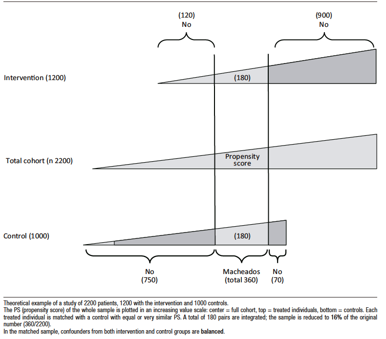
However, a significant number of individuals from both groups will be excluded because the corresponding pair is not available. The number of excluded individuals is directly related to the degree of confounder imbalance between the two groups in the original study sample. Thus, the conclusions of the trial and its application are limited to the matched sample and cannot be generalized to the entire population.
Inverse Probability of Treatment Weighting (IPTW)
Unlike matching, IPTW includes the entire sample under study.
While matching achieves adjustment by reducing the population until the confounders are equalized in the groups to be compared, IPTW achieves this objective by increasing the population with individuals who have a similar rate of confounders through a mathematical process.
Figure 4 shows a theoretical example that compares the intervention group with the control group. In this example platelet count is the only confounder considered, and it is dichotomized into > 105 mcL and ≤ 105 mcL).
There is an obvious imbalance, as there are three individuals in the treated group with platelets > 105 mcL and only one in the control group. The covariate platelets must be adjusted so that the two groups can be compared for a given outcome, for example, liver-related mortality or non-fatal gastrointestinal bleeding. For this purpose the PS in each is estimated.
If the matching strategy is applied, two pairs of 2 patients each, treated and control, sharing similar PS could be integrated: the sample would be limited to only four individuals (Figure 4).
In the same example, if the IPTW is used, the platelet covariate is adjusted by artificially increasing the number of observations, as previously mentioned, using the procedure detailed in Figure 5.
The PS is also used in the calculation, but in this case, by not reducing the number of observations, the result of the investigation can be generalized to a population that is more representative of real-world clinical practice.
However, in a real context, the probability of treatment is conditional to multiple confounders, whose overall effect is represented in the PS, which will differ for each individual (Figure 6). The procedure, similar to the one explained in Figure 5, although it reduces the imbalance, it is not perfect, and some differences persist in the distribution of individuals with thrombocytopenia between the treated and untreated groups, which is due to the effect of the other confounders.
The strategy detailed for platelets should be applied to all available variables or confounders considered when calculating PS.
Figure 4. Matching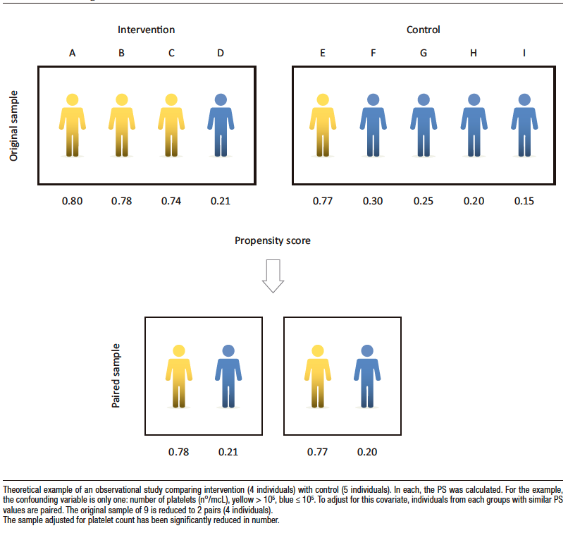
Figure 5. Inverse Probability of Treatment Weighting (IPTW)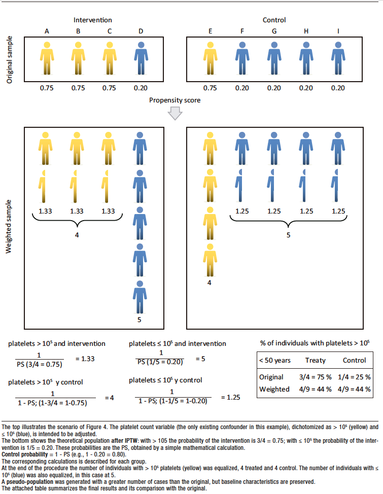
Figure 6. IPTW (Realistic Scenario)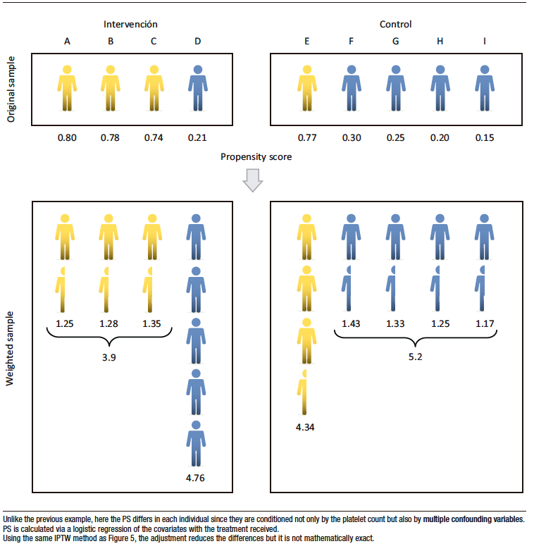
Estimating the Degree of Adjustment
Accurate adjustment is critical when applying the IPTW method to include all the individuals under study, as they will certainly have substantial differences in the prevalence of multiple confounders.
The standardized absolute difference (SAD), or the difference measured in standard deviation units, is typically used to assess the degree of adjustment achieved for each confounding variable after IPTW adjustment. Generally, it isaccepted that an adjustment is adequate if the difference is less than 0.10, although it sometimes extends to less than < 0.20, this detracts from the consistency of the study’s conclusions.
Figure 7 plots the SAD before and after adjustment to show the prior imbalance and the success of the procedure.
Figure 7. Evaluation of IPTW Adjustment in the Theoretical Trial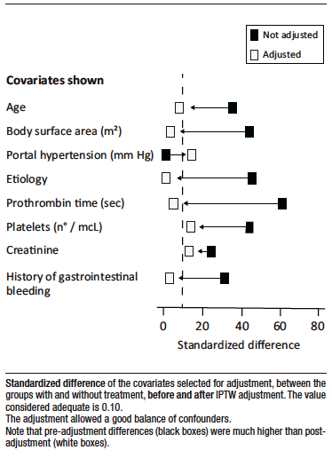
PS, IPTW, and Derived Analyses
The terms “propensity score” and “IPTW population” are frequently used in observational studies in the current medical literature, so it is necessary to understand the conceptual basis of these statistical methodologies.
The goal of both procedures is to create two populations that differ only in terms of whether or not they have received the intervention targeted by the study. This is because the rest of the conditioning variables that affect evolution have been “equalized.”
From here, one could continue with the statistical analysis by creating an adjusted Kaplan-Meier curve and using the Log-Rank Test or the Cox Model to estimate whether there is a significant difference between the groups.
Using the theoretical example of this paper, one could plot the relationship between the odds ratio of the outcome (e.g., liver-related mortality or non-fatal gastrointestinal bleeding) and different continuous covariates, such as platelet count, age, or prothrombin time. This would –allow one to consider the exact prognostic cut-off point.
An observational trial designed to evaluate an intervention or estimate the value of a prognostic index poses a methodological challenge. The key lies in the covariate adjustment procedure, which is used to determine the true value of the association under investigation.
The accuracy of PS in estimating the probability of intervention is a determining factor in the IPTW methodology. Once again, unmeasured or unknown confounders are a critical point of the statistical procedure.
Typically, a clinical study seeks to predict one variable (the dependent variable, endpoint, or outcome) from a set of independent variables, whether that prediction concerns present (diagnostic) or future (prognostic) outcomes. In any case, the outcome is conditioned by a multitude of these factors, which are statistically defined as independent variables.
However, a score can be generated from the outcome. For example, one could calculate the probability of gastrointestinal bleeding due to esophageal varices or mortality in chronic liver failure.
In other cases, it is of interest to know the effect of only one independent variable. If that variable is associated with others, known as confounding variables, the following question may arise: “Is the favorable outcome due to treatment effectiveness or it is because the treatment was indicated for individuals at lower risk?” In these cases, it’s necessary to isolate the association of interest from the confounders. This process is referred to as an adjustment in methodology. Randomized trials are the ideal option since confounders are balanced between groups when treatment is randomly assigned.
In observational studies, this problem is central and determines the outcome, whether the goal is assessing a prognostic indicator or to study the effect of an intervention. The applied methodology can include multivariate analysis, propensity score or inverse probability weighting. This statistical complexity affects the design and interpretation of bibliographic information.
In observational trials, necessary information comes from routine medical practice and is recorded in clinical histories or databases, sometimes international and large-scale (big data). Since it does not modify daily medical practice, it is clearly a true reflection of health care practice in the “real-world” and not an experimental condition, as occurs in randomized trials. This also explains the lower cost and feasibility of conducting the research.
The spectrum of methodological validity of an observational trial is broad. At one extreme is the recording of historical data from clinical histories, which often contains missing information or was obtained without a predefined, systematic approach. At the other extreme is a design with superior methodological value. This design requires an ad hoc protocol with a precise statistical methodology and other essential conditions. These conditions include specifying the inclusion and exclusion criteria, and defining the primary and secondary endpoints a priori, among other parameters.
The randomized versus observational trial option is false: both are complementary methodologies that advance medical knowledge.
What does deserve special consideration is the apt statement by physicist Richard Feynman: “It is much more interesting to live with uncertainty than to live with answers that might be wrong.”
Intellectual property. The authors declare that the data in the article are original and were carried out at their institutions.
Funding. The authors declare that there were no external sources of funding.
Conflict of interest. The authors declare that they have no competing interests related to this article.
Copyright

© 2025 Acta Gastroenterológica latinoamericana. This is an open-access article released under the terms of the Creative Commons Attribution (CC BY-NC-SA 4.0) license, which allows non-commercial use, distribution, and reproduction, provided the original author and source are acknowledged.
Cite this article as: Ciocca M, Mastai R y Cagide A. The Observational Study. Acta Gastroenterol Latinoam. 2025;55(2):79-87. https://doi.org/10.52787/agl.v55i2.489
Correspondence: Mirta Ciocca
Email: cioccamirta@gmail.com
Acta Gastroenterol Latinoam 2025;55(2):79-87